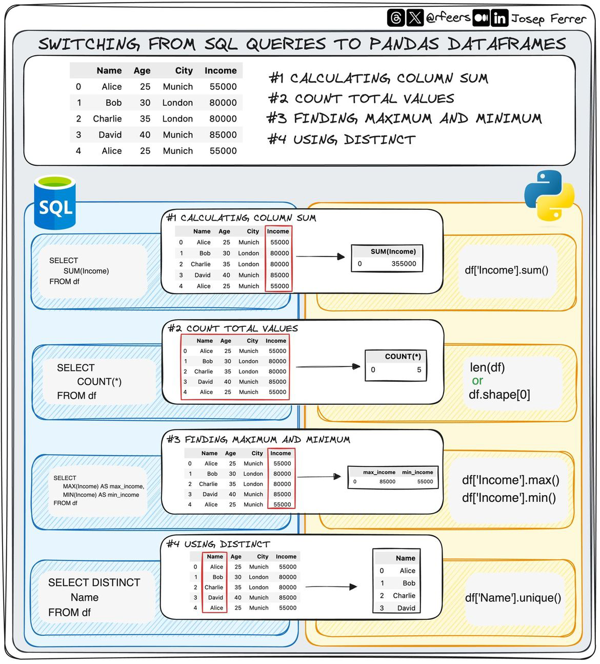
03: Join the DISTINCT with SQL
Links & Self-Guided Review
- DuckDB docs - embedded analytics database with strong CSV support
- JupySQL - SQL magics for notebooks
- SQL Style Guide (Mode) - readable query conventions
- SQLite docs - lightweight SQL reference
- PostgreSQL docs - production SQL dialect used widely in health systems
Outline
- Why SQL still runs the data world
- SQL in notebooks (JupySQL + DuckDB/SQLite)
- SQL basics: comments, NULLs, SELECT/WHERE
- Live demo 1
- SQL statement structure and execution order
- Importing data and defining tables
- Filtering and aggregation (WHERE vs HAVING)
- Joins, subqueries, CTEs, window functions
- Views, performance basics, SQL + Python workflows
- Live demo 2
- Live demo 3
Why SQL still runs the data world
SQL is how data teams ask precise questions of large relational datasets. In health data science, it shows up everywhere: EHR extracts, claims data, public health reporting, and analytics layers under dashboards.
| Where SQL shows up | What you use it for |
|---|---|
| EHR reporting | Cohorts, encounters, lab results |
| Claims data | Cost summaries, utilization, billing audits |
| Research datasets | Cleaning, joining, aggregating |
| Analytics stacks | ELT pipelines (extract → load → transform), dashboards, scheduled reports |

Reference Card: Why SQL matters
| Strength | Why it helps in practice |
|---|---|
| Declarative | You state what you want, not how to compute it |
| Scalable | Works on datasets larger than laptop RAM |
| Transferable | Similar syntax across DuckDB, SQLite, PostgreSQL |
| Composable | Queries can be layered and reused |
Code Snippet: Smallest useful query
SQL in notebooks (JupySQL + DuckDB/SQLite)
DuckDB is an embedded analytics database that feels like SQLite but is optimized for analytics. JupySQL lets you run SQL directly in notebooks using %sql for single-line and %%sql for multi-line queries, and it works with any SQLAlchemy-supported engine (SQLAlchemy is a Python toolkit for database connections).
JupySQL magics
Use %sql for quick, single-line queries and %%sql for multi-line blocks you want to read like a full query.
Reference Card: JupySQL magics
| Magic | Use case | Example |
|---|---|---|
%sql | Single-line query | %sql SELECT COUNT(*) FROM labs |
%%sql | Multi-line query | %%sql (cell header) |
Code Snippet: One-line query
DuckDB and SQLite connections
Both use lightweight file-based databases, so connection strings point to a local file and keep everything reproducible.
Reference Card: Local connections
| Engine | Connection string | Notes |
|---|---|---|
| DuckDB | duckdb:///clinic.db | Fast analytics on local files |
| SQLite | sqlite:///clinic.db | Portable file-based database |
Code Snippet: Connect to DuckDB
DuckDB + SQLite attachments
DuckDB can attach a SQLite database directly so you can query it without conversion. This is DuckDB-specific.
Reference Card: DuckDB SQLite attach
| Step | Purpose | Example |
|---|---|---|
| Install scanner | Load SQLite extension | INSTALL sqlite_scanner |
| Attach DB | Connect file | ATTACH 'chinook.sqlite' AS chinook (TYPE SQLITE) |
| List tables | Inspect schema | SHOW TABLES FROM chinook |
Code Snippet: Attach SQLite in DuckDB
INSTALL sqlite_scanner;
LOAD sqlite_scanner;
ATTACH 'chinook.sqlite' AS chinook (TYPE SQLITE);
SHOW TABLES FROM chinook;
Reference Card: Notebook setup
| Step | Command |
|---|---|
| Install | pip install duckdb duckdb-engine jupysql pandas |
| Load magic | %load_ext sql |
| Connect (DuckDB) | %sql duckdb:///clinic.duckdb |
| Connect (SQLite) | %sql sqlite:///clinic.sqlite |
| Return DataFrame | result = %sql SELECT * FROM table |
| Capture to variable | %%sql result << SELECT * FROM table |
Code Snippet: Minimal setup
Code Snippet: Return DataFrame (assignment)
Code Snippet: Return DataFrame (variable capture)
%%sql invoice_counts <<
SELECT BillingCountry, COUNT(*) AS invoice_count
FROM invoices
GROUP BY BillingCountry
ORDER BY invoice_count DESC
Querying DataFrames with SQL
DuckDB can query pandas DataFrames directly using replacement scans: use the DataFrame variable name in your SQL query. Replacement scans must be enabled when using SQLAlchemy connections (which JupySQL uses with connection strings).
Reference Card: DataFrame queries
| Pattern | Usage |
|---|---|
| Enable scans (required) | %sql SET python_scan_all_frames=true |
| Query DataFrame | %sql SELECT * FROM df WHERE x >= 5 |
| Capture result | %%sql result << SELECT * FROM df |
Code Snippet: Query a DataFrame
# Assume we already have duckdb connected and pandas imported
# Enable DataFrame replacement scans (required for SQLAlchemy connections)
%sql SET python_scan_all_frames=true

# Create a DataFrame
df = pd.DataFrame({
    'patient_id': [1, 2, 3, 4, 5],
    'age': [25, 30, 35, 40, 45],
    'department': ['Cardio', 'Neuro', 'Cardio', 'Neuro', 'Cardio']
})

# Query it with SQL (now works because replacement scans are enabled)
%sql SELECT department, COUNT(*) AS count FROM df GROUP BY department
SQL basics
These are the building blocks of most queries. Treat them as a checklist when reading or writing SQL.
Comments, semicolons, and NULLs
SQL statements end with semicolons, and comments start with --. NULL means missing, so comparisons need IS NULL rather than =.
| Value | Interpretation | Correct check |
|---|---|---|
NULL | Missing value | IS NULL / IS NOT NULL |
| Empty string | Present but blank | = '' |
| Zero | Numeric value | = 0 |
Reference Card: NULL handling
| Pattern | Example | Notes |
|---|---|---|
| Check missing | WHERE lab_value IS NULL | NULL is not equal to NULL |
| Fill missing | COALESCE(lab_value, 0) | Replace NULL with default |
| Safer filters | WHERE lab_value IS NOT NULL | Avoid accidental drops |
Code Snippet: NULL safe filtering
COALESCE
Use COALESCE to replace missing values with a default during queries.
Reference Card: COALESCE
| Function | Purpose | Example |
|---|---|---|
COALESCE | Fill NULLs | COALESCE(lab_value, 0) |
Code Snippet: Fill NULLs
SELECT, WHERE, ORDER BY, LIMIT, DISTINCT
This is the core of most queries: choose columns, filter rows, and order the output. Learn these first and most day-to-day SQL becomes readable.
| patient_id | encounter_date | department | total_cost |
|---|---|---|---|
| 2009 | 2024-03-06 | Cardiology | 560.00 |
| 2006 | 2024-03-01 | Emergency | 980.00 |
| 2010 | 2024-02-28 | Emergency | 1500.00 |
Reference Card: Core clauses
| Clause | Purpose | Example |
|---|---|---|
SELECT | Choose columns | SELECT patient_id, age |
WHERE | Filter rows | WHERE age >= 18 |
ORDER BY | Sort results | ORDER BY total_cost DESC |
LIMIT | Keep top N | LIMIT 10 |
DISTINCT | Unique values | SELECT DISTINCT department |
Reference Card: WHERE operators
| Operator | Purpose | Example |
|---|---|---|
| Comparisons | Match values | age >= 18 |
| Logical | Combine conditions | age >= 18 AND sex = 'F' |
IN | Match a set | department IN ('ER', 'ICU') |
BETWEEN | Match ranges | total_cost BETWEEN 100 AND 500 |
LIKE | Pattern match | test_name LIKE '%A1C%' |
Code Snippet: Basic filtering
SELECT encounter_id, patient_id, department, total_cost
FROM encounters
WHERE total_cost >= 500
ORDER BY total_cost DESC
LIMIT 5;
CASE WHEN
Use CASE WHEN to create conditional categories inside a query.
Reference Card: CASE WHEN
| Pattern | Purpose | Example |
|---|---|---|
CASE WHEN ... THEN ... END | Conditional logic | CASE WHEN age >= 65 THEN 'senior' ELSE 'adult' END |
Code Snippet: Conditional labels
SELECT patient_id,
    CASE
        WHEN age >= 65 THEN 'senior'
        WHEN age >= 18 THEN 'adult'
        ELSE 'minor'
    END AS age_group
FROM demographics;
COUNT(DISTINCT ...)
Use COUNT(DISTINCT ...) to count unique values instead of rows.
Reference Card: COUNT DISTINCT
| Pattern | Purpose | Example |
|---|---|---|
COUNT(DISTINCT col) | Unique count | COUNT(DISTINCT patient_id) |
Code Snippet: Unique patients per department
SELECT department, COUNT(DISTINCT patient_id) AS unique_patients
FROM encounters
GROUP BY department;
DISTINCT vs GROUP BY
Use DISTINCT for unique row combinations and GROUP BY when you need aggregates.
Reference Card: DISTINCT vs GROUP BY
| Tool | Best for | Example |
|---|---|---|
DISTINCT | Unique rows | SELECT DISTINCT department FROM encounters |
GROUP BY | Aggregation | SELECT department, COUNT(*) FROM encounters GROUP BY department |
Code Snippet: Unique departments
IN vs EXISTS
Use IN for small sets and EXISTS for correlated subqueries.
Reference Card: IN vs EXISTS
| Tool | Best for | Example |
|---|---|---|
IN | Small list or subquery | WHERE id IN (SELECT ...) |
EXISTS | Correlated checks | WHERE EXISTS (SELECT 1 ...) |
Code Snippet: EXISTS pattern
SELECT d.patient_id, d.age
FROM demographics AS d
WHERE EXISTS (
    SELECT 1
    FROM labs AS l
    WHERE l.patient_id = d.patient_id
);
LIKE vs ILIKE
Use LIKE for case-sensitive matching and ILIKE for case-insensitive matching when supported.
Reference Card: LIKE vs ILIKE
| Tool | Purpose | Example |
|---|---|---|
LIKE | Case-sensitive match | test_name LIKE '%A1C%' |
ILIKE | Case-insensitive match | test_name ILIKE '%a1c%' |
Code Snippet: Pattern matching
LIVE DEMO!
Importing data and defining tables
Real projects start with files. You can load CSVs directly, scan Parquet for columnar files (columnar means values are stored by column for faster analytics), or create tables with explicit types for safer analysis.
flowchart LR
    A[Raw CSV/Parquet files] --> B[Ingest (read_csv_auto / read_parquet)]
    B --> C[Typed table]
    C --> D[Query and reuse]
DuckDB read_csv_auto
read_csv_auto is DuckDB-specific and auto-detects column types for quick exploration.
Reference Card: read_csv_auto (DuckDB)
| Feature | Benefit | Example |
|---|---|---|
| Auto schema | Fast exploration | SELECT * FROM read_csv_auto('file.csv') |
Code Snippet: Quick CSV scan
DuckDB read_parquet
read_parquet is DuckDB-specific and reads columnar Parquet files efficiently.
Reference Card: read_parquet (DuckDB)
| Feature | Benefit | Example |
|---|---|---|
| Columnar reads | Faster analytics | SELECT * FROM read_parquet('file.parquet') |
Code Snippet: Parquet scan
COPY for bulk load
Use COPY when you need to ingest a large file quickly into a table.
Reference Card: COPY
| Option | Purpose | Example |
|---|---|---|
HEADER | Skip header row | HEADER true |
DELIMITER | Customize separator | DELIMITER ',' |
Code Snippet: COPY from CSV
COPY for exports
Use COPY ... TO when you want to write query results to CSV or Parquet.
Reference Card: COPY TO
| Format | Example | Notes |
|---|---|---|
| CSV | COPY (...) TO 'file.csv' (HEADER) | Easy to inspect |
| Parquet | COPY (...) TO 'file.parquet' (FORMAT PARQUET) | Efficient analytics |
Code Snippet: Export to CSV and Parquet
COPY (SELECT * FROM demographics LIMIT 100)
TO 'demographics_sample.csv' (HEADER, DELIMITER ',');

COPY (SELECT * FROM demographics LIMIT 100)
TO 'demographics_sample.parquet' (FORMAT PARQUET);
CREATE TABLE AS COPY
Create and populate a table in one step when you want an explicit schema.
Reference Card: CREATE TABLE AS COPY
| Benefit | Use case |
|---|---|
| Single step | Reproducible loads |
| Explicit types | Safer analysis |
Code Snippet: Create table + load
CREATE TABLE demographics (
    patient_id INTEGER,
    age INTEGER,
    sex TEXT
) AS COPY FROM 'demographics.csv'
WITH (FORMAT CSV, HEADER true);
Reference Card: Common import patterns
| Pattern | Use case | Example |
|---|---|---|
read_csv_auto | Quick CSV exploration | SELECT * FROM read_csv_auto('file.csv') |
read_parquet | Fast columnar reads | SELECT * FROM read_parquet('file.parquet') |
CREATE TABLE AS | Persist results | CREATE TABLE t AS SELECT ... |
COPY | Fast bulk load | COPY t FROM 'file.csv' (HEADER true) |
Code Snippet: Create table from CSV
Filtering and aggregation
Filtering shrinks the data to what you need. Aggregation summarizes it to the level you want to report. Use WHERE to filter rows before grouping and HAVING to filter groups after aggregation; if you are unsure, start with WHERE.
WHERE vs HAVING
WHERE filters raw rows, and HAVING filters aggregated groups after GROUP BY.
Reference Card: WHERE vs HAVING
| Clause | Applies to | Example |
|---|---|---|
WHERE | Rows before grouping | WHERE total_cost > 500 |
HAVING | Groups after GROUP BY | HAVING COUNT(*) > 3 |
GROUP BY and aggregates
Aggregates like COUNT and AVG summarize each group into a single row of results.
Reference Card: Aggregates
| Function | Purpose | Example |
|---|---|---|
COUNT | Row counts | COUNT(*) |
AVG | Mean | AVG(total_cost) |
SUM | Totals | SUM(total_cost) |
flowchart LR
    A[Raw rows] --> B[WHERE filters rows]
    B --> C[GROUP BY aggregates]
C --> D[HAVING filters groups]| Department | Visit count | Avg cost |
|---|---|---|
| Cardiology | 7 | 812.50 |
| Oncology | 5 | 1230.20 |
| Primary Care | 12 | 210.30 |
Reference Card: Filtering + aggregates
| Tool | Example | Purpose |
|---|---|---|
GROUP BY | GROUP BY department | Define groups |
HAVING | HAVING COUNT(*) > 3 | Filter groups |
| Aggregates | COUNT, AVG, SUM | Summarize |
Code Snippet: Filter then group
SELECT department,
    COUNT(*) AS visit_count,
    AVG(total_cost) AS avg_cost
FROM encounters
WHERE encounter_date >= '2024-01-01'
GROUP BY department
ORDER BY avg_cost DESC;
ROUND
Use ROUND to tidy numeric summaries for reporting after you aggregate.
Reference Card: ROUND
| Function | Purpose | Example |
|---|---|---|
ROUND | Set decimal places | ROUND(AVG(total_cost), 2) |
Code Snippet: Rounded averages

Joins: combine tables safely
Joins connect demographics, encounters, and lab results. Always join on keys and check for row explosion (many-to-many joins can multiply rows).
Joins
Plan joins like data links: define the primary key, check duplicates, and test row counts before and after.
Reference Card: Join checks
| Check | Why it matters | Quick test |
|---|---|---|
| Key uniqueness | Prevent row explosion | COUNT(*) vs COUNT(DISTINCT key) |
| Row counts | Detect unexpected growth | Compare counts pre/post join |
Code Snippet: Pre-join key check
Join types
Join type determines which rows survive when keys are missing or unmatched.

Reference Card: Join types
| Join | Keeps rows from | When to use |
|---|---|---|
INNER JOIN | Both tables | Only matched records |
LEFT JOIN | Left table | Keep all patients, add matches |
RIGHT JOIN | Right table | Rare in analytics |
FULL JOIN | Both tables | Audits, reconciliation |
Code Snippet: Encounter + demographics
SELECT e.encounter_id, e.department, d.age, d.sex
FROM encounters AS e
LEFT JOIN demographics AS d
    ON e.patient_id = d.patient_id;
ON vs USING
Use ON when columns differ in name or you need a more complex condition. Use USING when column names match and you want a cleaner query.
Reference Card: ON vs USING
| Syntax | Best for | Example |
|---|---|---|
ON | Different column names or conditions | ON e.patient_id = d.patient_id |
USING | Same column name in both tables | USING (patient_id) |
Code Snippet: USING clause
flowchart LR
    A[encounters.patient_id] -->|ON e.patient_id = d.patient_id| C[Join]
    B[demographics.patient_id] -->|USING (patient_id)| C
UNION ALL
Use UNION ALL to stack compatible result sets without de-duplicating rows.
Reference Card: UNION ALL
| Operator | Purpose | Example |
|---|---|---|
UNION ALL | Stack results | SELECT ... UNION ALL SELECT ... |
Code Snippet: Stack row counts
SELECT 'encounters' AS table_name, COUNT(*) AS rows FROM encounters
UNION ALL
SELECT 'labs', COUNT(*) FROM labs
ORDER BY table_name;
SQL statement structure and execution order
SQL reads like English, but it executes in a specific order. When a query is confusing, rewrite it as a pipeline: join tables, filter rows, group, compute, then sort.
Statement structure
Write SQL in the order you want it to read: SELECT what you want, FROM where it lives, and WHERE how you filter.
Reference Card: Readable structure
| Step | Purpose | Example |
|---|---|---|
SELECT | Choose columns | SELECT patient_id, age |
FROM | Pick table | FROM demographics |
WHERE | Filter rows | WHERE age >= 18 |
Code Snippet: Skeleton query
Execution order
Execution happens from FROM/JOIN to WHERE to GROUP BY, then SELECT and ORDER BY, which explains why aliases are sometimes unavailable in WHERE.
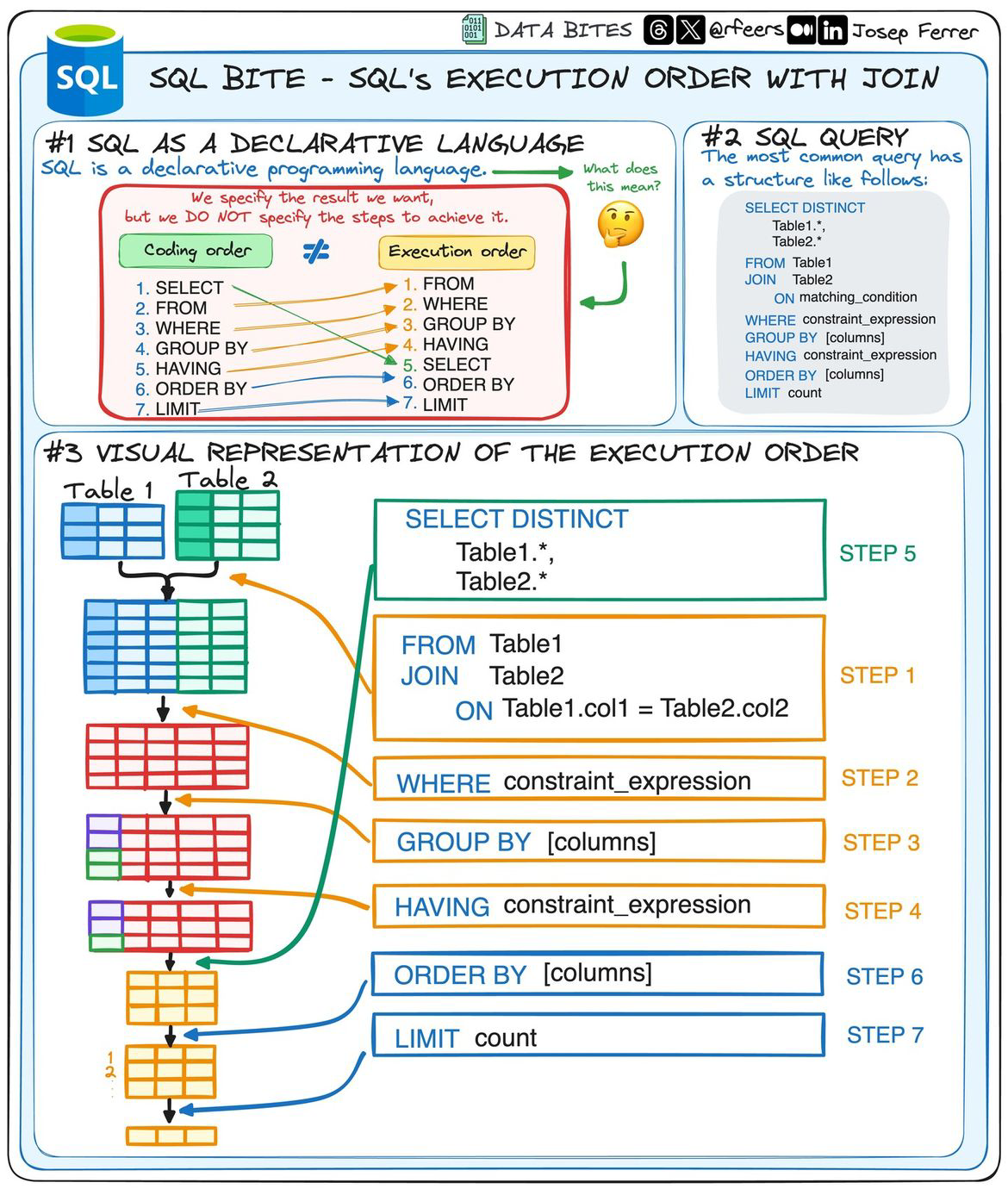
Read a query top to bottom in this order:
- Build tables with
FROM+JOIN - Filter rows with
WHERE - Aggregate with
GROUP BYand filter groups withHAVING - Compute output with
SELECT - Sort and trim with
ORDER BY+LIMIT
Reference Card: Execution order (simplified)
| Order | Clause |
|---|---|
| 1 | FROM + JOIN |
| 2 | WHERE |
| 3 | GROUP BY |
| 4 | HAVING |
| 5 | SELECT |
| 6 | ORDER BY |
| 7 | LIMIT |
Code Snippet: Readable query template
SELECT department, COUNT(*) AS visit_count
FROM encounters
WHERE total_cost > 500
GROUP BY department
HAVING COUNT(*) >= 3
ORDER BY visit_count DESC
LIMIT 5;
LIVE DEMO!!
Subqueries and CTEs
Subqueries let you nest logic. CTEs (WITH) make that logic readable and reusable, which matters for multi-step cohort definitions (a cohort is a defined group of patients).
Subqueries
Use a subquery when you need a compact, one-off filter or calculation inside a larger query.
Reference Card: Subqueries
| Pattern | Use case | Example |
|---|---|---|
IN (SELECT ...) | Filter by a derived set | WHERE id IN (SELECT ...) |
| Scalar subquery | Single value in SELECT | (SELECT MAX(...)) |
Code Snippet: Subquery filter
SELECT patient_id, age
FROM demographics
WHERE patient_id IN (
    SELECT patient_id
    FROM labs
    WHERE test_name = 'A1C' AND value >= 7.0
);
CTEs
Use a CTE when the logic has multiple steps or needs to stay readable across several joins or filters.
Reference Card: CTEs
| Feature | Benefit | Example |
|---|---|---|
WITH name AS (...) | Reuse readable steps | WITH cohort AS (...) |
flowchart LR
    A[Main query] --> B[Inline subquery]
    A --> C[CTE: WITH cohort AS (...)]
    C --> D[Main query uses cohort]
Reference Card: Subqueries vs CTEs
| Pattern | Best for | Example |
|---|---|---|
| Subquery | Small, single use logic | WHERE id IN (SELECT ...) |
| CTE | Multi-step, readable logic | WITH cohort AS (...) |
Code Snippet: CTE for a cohort
WITH high_a1c AS (
    SELECT patient_id
    FROM labs
    WHERE test_name = 'A1C' AND value >= 7.0
)
SELECT d.patient_id, d.age, d.sex
FROM demographics AS d
INNER JOIN high_a1c AS h
    ON d.patient_id = h.patient_id;
Window functions
Window functions compute metrics across related rows without collapsing them. They are common in claims and encounter analytics (running totals, most recent visit, rank within a patient).
| patient_id | encounter_date | total_cost | running_cost |
|---|---|---|---|
| 101 | 2024-01-10 | 220.00 | 220.00 |
| 101 | 2024-02-03 | 125.00 | 345.00 |
| 101 | 2024-03-02 | 410.00 | 755.00 |
Reference Card: Window function patterns
| Function | Use case | Example |
|---|---|---|
ROW_NUMBER | Order rows | ROW_NUMBER() OVER (...) |
LAG | Compare to previous | LAG(total_cost) |
SUM | Running totals | SUM(total_cost) OVER (...) |
Code Snippet: Running total per patient
SELECT patient_id,
    encounter_date,
    total_cost,
    SUM(total_cost) OVER (
        PARTITION BY patient_id
        ORDER BY encounter_date
    ) AS running_cost
FROM encounters
ORDER BY patient_id, encounter_date;

Data modification (INSERT, UPDATE, DELETE)
These statements change data in place. Use them sparingly in analytics and favor scratch databases when you need to write.
flowchart LR
    A[SELECT preview] --> B[INSERT/UPDATE/DELETE]
    B --> C[Validate row counts]
    C --> D[Commit or rollback]
Reference Card: Data modification statements
| Statement | Use case | Guardrail |
|---|---|---|
INSERT | Add rows | Use explicit column lists |
UPDATE | Edit rows | Always include a WHERE |
DELETE | Remove rows | Preview with SELECT first |
INSERT
Use explicit column lists and treat inserts as append-only in analytics workflows.
Code Snippet: Safe insert
UPDATE
Always include a WHERE and check the affected rows before committing the change.
Reference Card: UPDATE
| Guardrail | Why it helps |
|---|---|
WHERE required | Prevents full-table edits |
| Preview first | Confirms target rows |
Code Snippet: Safe update
DELETE
Preview the rows with a SELECT first, then delete with the same WHERE filter.
Reference Card: DELETE
| Guardrail | Why it helps |
|---|---|
Preview with SELECT | Validate target rows |
| Limit scope | Avoid accidental full delete |
Code Snippet: Targeted delete
CAST
Use CAST to convert types explicitly before comparisons or aggregations.
Reference Card: CAST
| Function | Purpose | Example |
|---|---|---|
CAST | Convert types | CAST(encounter_date AS DATE) |
Code Snippet: Cast to DATE
SELECT CAST(encounter_date AS DATE) AS visit_date, COUNT(*) AS visits
FROM encounters
GROUP BY CAST(encounter_date AS DATE)
ORDER BY visit_date;
date_part
Use date_part to extract date pieces for grouping and filtering.
Reference Card: date_part
| Function | Purpose | Example |
|---|---|---|
date_part | Extract date parts | date_part('month', encounter_date) |
Code Snippet: Group by month
SELECT date_part('month', encounter_date) AS month, COUNT(*) AS visits
FROM encounters
GROUP BY month
ORDER BY month;
DATE_TRUNC
Use DATE_TRUNC to bucket timestamps into consistent time windows.
Reference Card: DATE_TRUNC
| Function | Purpose | Example |
|---|---|---|
DATE_TRUNC | Time buckets | DATE_TRUNC('month', encounter_date) |
Code Snippet: Monthly buckets
SELECT DATE_TRUNC('month', encounter_date) AS month, COUNT(*) AS visits
FROM encounters
GROUP BY month
ORDER BY month;
Views and materialized views
Views save a query definition. Materialized views store a cached snapshot of results, which can speed up dashboards at the cost of refresh time.
Views
Use views to keep a canonical definition of common queries without duplicating SQL logic.
Reference Card: Views
| Property | Notes |
|---|---|
| Stored data | No |
| Refresh | Always current |
Materialized views
Use materialized views when you can afford scheduled refreshes in exchange for faster reads.
Reference Card: Materialized views
| Property | Notes |
|---|---|
| Stored data | Yes |
| Refresh | Manual or scheduled |
flowchart LR
    A[Query definition] --> B[View (no stored data)]
    A --> C[Materialized view (stored snapshot)]
    C --> D[Refresh schedule]
Code Snippet: Create a view
CREATE VIEW high_cost_encounters AS
SELECT encounter_id, patient_id, total_cost
FROM encounters
WHERE total_cost >= 1000;
Code Snippet: Create a materialized view
CREATE MATERIALIZED VIEW high_cost_encounters_mv AS
SELECT encounter_id, patient_id, total_cost
FROM encounters
WHERE total_cost >= 1000;
Performance basics
Performance depends on reading less data and doing work once. A query plan is the database's step-by-step execution order; start with filters and clear joins before reaching for complex optimizations.
flowchart LR
    A[Query] --> B[EXPLAIN plan]
    B --> C[Find slow step]
    C --> D[Optimize: filter, index, join]
Reference Card: Performance checklist
| Tip | Why it helps |
|---|---|
| Filter early | Less data to join and aggregate |
| Select only needed columns | Reduces memory usage |
| Use indexes (when supported) | Faster lookups |
| Inspect query plans | Find slow steps |
Code Snippet: Explain a query
SQL + Python workflows
SQL is great for filtering and aggregation; Python is great for modeling and visualization. Use SQL to reduce the dataset, then load the result into pandas for analysis. DuckDB and SQLite are easy local options; for external databases, connect via SQLAlchemy and reuse the same query strings.
SQL for reduction
Use SQL to filter to cohorts, aggregate to reporting levels, and shrink the data before it hits memory.
Reference Card: Reduction patterns
| Pattern | Goal | Example |
|---|---|---|
| Filter | Keep cohort | WHERE age >= 18 |
| Aggregate | Summarize | GROUP BY department |
Code Snippet: Reduce before pandas
SELECT department, COUNT(*) AS visit_count
FROM encounters
WHERE encounter_date >= '2024-01-01'
GROUP BY department;
Python for analysis
Load the reduced dataset into pandas for plots, modeling, and downstream feature engineering.
Reference Card: pandas entry points
| Method | When to use |
|---|---|
pd.read_sql | SQLAlchemy connections |
fetch_df | DuckDB result to DataFrame |
Code Snippet: pandas from SQLAlchemy
SQLite connections
Use SQLite for lightweight, file-based workflows that still support standard SQL.
Reference Card: SQLite
| Tool | Usage |
|---|---|
sqlite3.connect | sqlite3.connect("clinic.db") |
pd.read_sql_query | pd.read_sql_query(query, conn) |
Code Snippet: SQLite to pandas
import sqlite3
import pandas as pd

conn = sqlite3.connect("clinic.db")
query = "SELECT department, COUNT(*) AS visit_count FROM encounters GROUP BY department"
report = pd.read_sql_query(query, conn)
| Step | Tool | Output |
|---|---|---|
| Query | SQL | Table of filtered rows |
| Analyze | pandas | DataFrame, plots |
| Model | sklearn | Features, predictions |
Reference Card: pandas interop
| Method | Usage |
|---|---|
pd.read_sql | pd.read_sql(query, connection) |
| DuckDB to pandas | duckdb.sql(query).df() |
| Save results | df.to_parquet("outputs/report.parquet") |
Code Snippet: SQLAlchemy connection
import pandas as pd
from sqlalchemy import create_engine

engine = create_engine("postgresql://user:password@localhost:5432/clinic")
query = "SELECT department, COUNT(*) AS visit_count FROM encounters GROUP BY department"
report = pd.read_sql(query, engine)
Code Snippet: SQL to DataFrame
import duckdb
import pandas as pd

con = duckdb.connect("clinic.db")
query = """
SELECT department, COUNT(*) AS visit_count
FROM encounters
GROUP BY department
"""
report = con.execute(query).fetch_df()
print(report.head())
LIVE DEMO!!!
Advanced SQL patterns (optional)
These patterns are useful in production analytics but are not required for the demos.
NULLIF for safe division
Use NULLIF to avoid divide-by-zero errors in ratios.
Reference Card: NULLIF
| Function | Purpose | Example |
|---|---|---|
NULLIF | Return NULL on match | NULLIF(denominator, 0) |
Code Snippet: Safe rate
ORDER BY NULLS FIRST/LAST
Some dialects let you control where NULLs appear in sorted results.
Reference Card: NULL ordering
| Clause | Purpose | Example |
|---|---|---|
NULLS FIRST | NULLs at top | ORDER BY lab_value NULLS FIRST |
NULLS LAST | NULLs at end | ORDER BY lab_value NULLS LAST |
Code Snippet: Explicit NULL ordering
LIMIT and OFFSET
Use pagination to fetch results in smaller chunks.
Reference Card: Pagination
| Clause | Purpose | Example |
|---|---|---|
LIMIT | Cap rows | LIMIT 50 |
OFFSET | Skip rows | OFFSET 100 |
Code Snippet: Page through results
INSERT ... SELECT
Use query results to populate another table.
Reference Card: INSERT SELECT
| Pattern | Purpose | Example |
|---|---|---|
INSERT ... SELECT | Load from query | INSERT INTO t SELECT ... |
Code Snippet: Insert cohort
UPDATE ... FROM
Use joins to update rows based on another table.
Reference Card: UPDATE FROM
| Pattern | Purpose | Example |
|---|---|---|
UPDATE ... FROM | Join-based update | UPDATE t SET ... FROM s WHERE ... |